Forecasting Mortality Rates Using a Stochastic PCA–GEE Model: Single Population Analysis

Authors

Reza Dastranj

Martin Kolář

Published

October 29, 2025

Introduction

This document presents an analysis of mortality rate forecasting for single populations using Principal Component Analysis (PCA) combined with Generalized Estimating Equations (GEEs).
The performance of this hybrid PCA–GEE framework is compared with the traditional demographic Lee–Carter (LC) model across 56 populations from the Human Mortality Database (HMD).

1. Loading Required Packages

The following R packages are required for data handling, statistical modeling, and visualization.

# --- Essential Libraries ---
library(data.table)     # Fast data manipulation
library(dplyr)          # Data wrangling and pipes
library(ggplot2)        # Visualization
library(HMDHFDplus)     # import HMD data
library(forecast)       # Time series forecasting rwf
library(geepack)        # GEE modeling

# --- Setup ---
theme_set(theme_bw())   # Set default plotting theme
set.seed(1242)          # Ensure reproducibility

2. Data Import

Importing downloaded datasets from the Human Mortality Database (HMD) website. Data source: Human Mortality Database. Licensed under CC BY 4.0.

Mortality data are imported from the HMD for 56 populations (both genders). The datasets include mortality rates (mx) by age and year.

mylistmf<-c(
  "AUS.fltper_1x1.txt","AUT.fltper_1x1.txt","BEL.fltper_1x1.txt",
  "BGR.fltper_1x1.txt"                     ,"CAN.fltper_1x1.txt",
  "CHE.fltper_1x1.txt","CZE.fltper_1x1.txt",
  "DEUTE.fltper_1x1.txt","DEUTW.fltper_1x1.txt","DNK.fltper_1x1.txt",
  "ESP.fltper_1x1.txt","FIN.fltper_1x1.txt",
  "FRATNP.fltper_1x1.txt","GBR_NIR.fltper_1x1.txt","GBR_NP.fltper_1x1.txt",
  "GBR_SCO.fltper_1x1.txt","GBRTENW.fltper_1x1.txt",
  "HUN.fltper_1x1.txt","IRL.fltper_1x1.txt",
  "ISL.fltper_1x1.txt","ITA.fltper_1x1.txt",
  "JPN.fltper_1x1.txt",
  "NLD.fltper_1x1.txt","NOR.fltper_1x1.txt",
  "PRT.fltper_1x1.txt",
  "SVK.fltper_1x1.txt",
  "SWE.fltper_1x1.txt",
  "USA.fltper_1x1.txt",
  "AUS.mltper_1x1.txt","AUT.mltper_1x1.txt","BEL.mltper_1x1.txt",
  "BGR.mltper_1x1.txt"                     ,"CAN.mltper_1x1.txt",
  "CHE.mltper_1x1.txt","CZE.mltper_1x1.txt",
  "DEUTE.mltper_1x1.txt","DEUTW.mltper_1x1.txt","DNK.mltper_1x1.txt",
  "ESP.mltper_1x1.txt","FIN.mltper_1x1.txt",
  "FRATNP.mltper_1x1.txt","GBR_NIR.mltper_1x1.txt","GBR_NP.mltper_1x1.txt",
  "GBR_SCO.mltper_1x1.txt","GBRTENW.mltper_1x1.txt",
  "HUN.mltper_1x1.txt","IRL.mltper_1x1.txt",
  "ISL.mltper_1x1.txt","ITA.mltper_1x1.txt",
  "JPN.mltper_1x1.txt",
  "NLD.mltper_1x1.txt","NOR.mltper_1x1.txt",
  "PRT.mltper_1x1.txt",
  "SVK.mltper_1x1.txt",
  "SWE.mltper_1x1.txt",
  "USA.mltper_1x1.txt"
)

3. Lee–Carter Model for 56 Single Populations

The Lee–Carter (LC) model is applied to each population to estimate and forecast log-mortality rates. Model performance is assessed via Mean Squared Error (MSE) for testing periods.

# ============================================================
# Lee–Carter Model for Forecasting Mortality Rates
# ============================================================
# This section implements the Lee–Carter (LC) model for 56 single populations
# from the HMD. The model decomposes the
# log-mortality surface into age, time, and residual components.
# Forecasting is performed via a random walk with drift.
# ============================================================

# Initialize a vector to store test MSEs

MSE_test_lc  <- c()

# ------------------------------------------------------------
# Loop through all 56 populations (28 countries × 2 genders)
# ------------------------------------------------------------
for (n in 1:56) {
  
  # ------------------------------------------------------------
  # STEP 1: Load and preprocess mortality data
  # ------------------------------------------------------------
  dat <- HMDHFDplus::readHMD(mylistmf[n]) %>% data.table()
  
  # Replace zero mortality rates with a small constant to avoid log(0)
  dat$mx[dat$mx == 0] <- 0.000004
  
  # Compute log-mortality
  dat[, logmx := log(mx)]
  
  # Filter the data: include years ≥ 1961 and ages ≤ 90
  dat <- dat[Year >= 1961 & Age <= 90]
  
  # ------------------------------------------------------------
  # STEP 2: Prepare data for the LC model
  # ------------------------------------------------------------
  t <- 50  # Number of years in the training period (1961–2010)
  
  # Subset training data (up to 2010)
  dat_train <- dat[Year <= 2010]
  
  # Create a matrix of log-mortality rates by year (rows) and age (columns)
  M <- matrix(dat_train$logmx, nrow = t, ncol = 91, byrow = TRUE)
  
  # Compute average log-mortality by age (the 'a_x' term in LC model)
  a <- colMeans(M)
  
  # Center the log-mortality matrix by subtracting the mean at each age
  for (j in 1:91) M[, j] <- M[, j] - a[j]
  
  # ------------------------------------------------------------
  # STEP 3: Singular Value Decomposition (SVD)
  # ------------------------------------------------------------
  # SVD decomposes M ≈ a_x + b_x * k_t, capturing age–time interaction.
  d <- svd(M, nu = 1, nv = 1)  # Extract the first singular component
  
  # Normalize the age-specific sensitivity vector (b_x)
  b <- d$v / sum(d$v)
  
  # Compute the time-varying mortality index (k_t)
  k <- d$u * sum(d$v) * d$d[1]
  
  # ------------------------------------------------------------
  # STEP 4: Model the time series of k_t
  # ------------------------------------------------------------
  # The Lee–Carter model assumes k_t follows a random walk with drift.
  RW <- k
  
  # Estimate the drift term from the first-difference of k_t
  incpt1 <- round(mean(arima(diff(RW), order = c(0, 0, 0))$coef), 7)
  
  # Determine forecast horizon (number of years to predict)
  tsty <- length(unique(dat$Year)) - t
  
  # ------------------------------------------------------------
  # STEP 5: Forecast k_t using random walk with drift
  # ------------------------------------------------------------
  k_forecast <- k
  for (j in 1:tsty) {
    k_forecast <- append(k_forecast, RW[t] + j * incpt1)
  }
  
  # ------------------------------------------------------------
  # STEP 6: Reconstruct fitted and forecasted log-mortality
  # ------------------------------------------------------------
  # Compute fitted log-mortality values for both training and test periods
  lc_fit <- sapply(1:(t + tsty), function(i) a + b * k_forecast[i])
  
  # Convert to matrix form: rows = years, columns = ages
  lc_fit_matrix <- matrix(lc_fit, nrow = t + tsty, ncol = 91, byrow = TRUE)
  
  # ------------------------------------------------------------
  # STEP 7: Compute Model Errors (Training and Test)
  # ------------------------------------------------------------
  # Create full log-mortality matrix (training + test)
  N <- matrix(dat$logmx, nrow = t + tsty, ncol = 91, byrow = TRUE)
  
  # Calculate model residuals on the mortality scale
  Error_LC <- exp(N) - exp(lc_fit_matrix)
  
  # Mean Squared Error for testing period (post-2010)
  MSE_test  <- sum(Error_LC[(t + 1):(t + tsty), ]^2) / (91 * tsty)
  
  # Append results
  MSE_test_lc  <- append(MSE_test_lc, MSE_test)
}

# ------------------------------------------------------------
# STEP 8: Output test MSE for all populations
# ------------------------------------------------------------
MSE_test_lc

 [1] 1.261742e-06 5.745571e-06 4.180935e-06 9.101754e-05 1.651217e-06
 [6] 1.234632e-05 1.590203e-05 4.369004e-06 1.927844e-06 1.008191e-05
[11] 2.763997e-06 4.728147e-06 2.550245e-06 1.535708e-05 3.276198e-06
[16] 2.825327e-05 3.151300e-06 8.514082e-06 5.986238e-06 9.529308e-06
[21] 8.487293e-06 1.829712e-06 9.523191e-06 6.955758e-06 4.713238e-06
[26] 1.397978e-05 1.606216e-06 7.919542e-06 1.410023e-05 9.441788e-06
[31] 2.959573e-05 2.096039e-04 2.558052e-05 6.022354e-06 2.423164e-05
[36] 6.624540e-06 7.988849e-06 1.563310e-05 9.537184e-06 1.082463e-05
[41] 3.415690e-06 1.268257e-05 9.665005e-06 1.587764e-05 9.999469e-06
[46] 5.617536e-05 9.407608e-05 6.669273e-05 1.078205e-05 3.541542e-06
[51] 5.155572e-05 5.853514e-05 5.246112e-06 1.111074e-04 1.439767e-05
[56] 8.807678e-06

4. Stochastic PCA–GEE Model

The Stochastic PCA–GEE model introduces dimension reduction through PCA, followed by a GEE structure to capture correlations within age groups.

# ============================================================
# 4. Stochastic PCA–GEE Model
# ============================================================
# This section applies Principal Component Analysis (PCA)
# in combination with Generalized Estimating Equations (GEEs)
# to model and forecast age-specific mortality rates.
# ============================================================

# Initialize an empty vector to store test MSE values for each population

MSE_test_gee <- c()

# Loop through all 56 populations (28 countries × 2 genders)
for (n in 1:56) {
  
  # ------------------------------------------------------------
  # STEP 1: Load and preprocess mortality data
  # ------------------------------------------------------------
  dat0 <- HMDHFDplus::readHMD(mylistmf[n]) %>% data.table()
  
  # Replace zero mortality values with a small constant to avoid log(0)
  dat0$mx[dat0$mx == 0] <- 0.000004
  
  # Compute log mortality rate
  dat0[, logmx := log(mx)]
  
  # Keep years ≥ 1961 and ages ≤ 90 for consistent modeling
  dat0 <- dat0[Year >= 1961 & Age <= 90]
  
  # Create a matrix of log mortality rates
  M0 <- matrix(dat0$logmx, length(unique(dat0$Year)), 91, byrow = TRUE)
  
  # Subset data for training period (1961–2010)
  dat <- dat0[Year <= 2010]
  M <- matrix(dat$logmx, 50, 91, byrow = TRUE)  # 50 years (training)
  
  # ------------------------------------------------------------
  # STEP 2: Apply PCA by age groups to extract the main components
  # ------------------------------------------------------------
  # The age range (0–90) is divided into 3 groups:
  #   1. 0–14  (15 ages)
  #   2. 15–40 (26 ages)
  #   3. 41–90 (50 ages)
  # For each group, the first principal component is extracted.
  
  kcList <- list()
  
  # Compute the first PC for each age segment
  result1 <- rep(prcomp(M[, 1:15], center = FALSE, scale. = FALSE)$x[, 1], times = 15)
  result2 <- rep(prcomp(M[, 16:41], center = FALSE, scale. = FALSE)$x[, 1], times = 26)
  result3 <- rep(prcomp(M[, 42:91], center = FALSE, scale. = FALSE)$x[, 1], times = 50)
  
  # Combine results into a single list and flatten
  kcList <- c(kcList, c(result1, result2, result3))
  kc1 <- unlist(kcList)     # Principal component scores (flattened)
  kc2 <- kc1^2              # Square of the component scores for non-linearity
  
  # ------------------------------------------------------------
  # STEP 3: Prepare data for GEE model training
  # ------------------------------------------------------------
  t <- 50
  year <- rep(1961:2010, times = 91)
  age <- rep(0:90, each = t)
  cohort <- year - age
  
  ASDRs <- data.frame(
    kc1 = kc1,
    kc2 = kc2,
    cohort = cohort,
    y = as.vector(M),
    age = factor(age, levels = 0:90),
    year = year,
    stringsAsFactors = FALSE
  )
  
  # Add numeric age for weighting and use as subject ID for correlation
  ASDRs$agenum <- as.numeric(ASDRs$age)
  ASDRs$subject <- ASDRs$age
  
  # ------------------------------------------------------------
  # STEP 4: Fit GEE model with AR(1) correlation structure
  # ------------------------------------------------------------
  # The model links log-mortality (y) to age, age × PCA interactions.
  # Within each age group, correlations across time are modeled using AR(1).
  
  geeAr1 <- geepack::geeglm(
    y ~ -1 + age + age:kc1,
    data = ASDRs,
    id = subject,
    waves = year,
    corstr = "ar1",
    weights = agenum / mean(agenum)
  )
  
  # Store fitted values for training data
  ASDRs$fit <- predict(geeAr1, ASDRs)
  
  # ------------------------------------------------------------
  # STEP 5: Forecast principal component time series (Random Walk with Drift)
  # ------------------------------------------------------------
  # For each PCA segment, the time series of component scores is extended
  # to forecast future years (post-2010) up to the maximum available year.
  
  kcList <- list()
  kc0 <- c(
    prcomp(M[, 1:15], center = FALSE, scale. = FALSE)$x[, 1],
    prcomp(M[, 16:41], center = FALSE, scale. = FALSE)$x[, 1],
    prcomp(M[, 42:91], center = FALSE, scale. = FALSE)$x[, 1]
  )
  
  # Forecast horizon (number of test years)
  tsty <- length(unique(dat0$Year)) - 50
  
  ar <- c()
  for (i in 1:3) {
    # Extract each PC segment and forecast future values
    subset_kc0 <- kc0[((i - 1) * 50 + 1):(i * 50)]
    kc_forecast <- forecast::rwf(subset_kc0, h = tsty, drift = TRUE)
    ar <- append(ar, kc_forecast$mean[1:tsty])
  }
  
  # Replicate forecasted PC values across age ranges
  result1 <- rep(ar[1:tsty], times = 15)
  result2 <- rep(ar[(tsty + 1):(2 * tsty)], times = 26)
  result3 <- rep(ar[(2 * tsty + 1):(3 * tsty)], times = 50)
  kc1 <- c(result1, result2, result3)
  kc2 <- kc1^2
  
  # ------------------------------------------------------------
  # STEP 6: Construct test dataset and make GEE-based predictions
  # ------------------------------------------------------------
 
  
  year <- rep(2011:max(dat0$Year), times = 91)
  age <- rep(0:90, each = tsty)
  cohort <- year - age
  
  newASDRs <- data.frame(
    kc1 = kc1,
    kc2 = kc2,
    cohort = cohort,
    y = as.vector(M0[51:(50 + tsty), ]),
    age = factor(age, levels = 0:90),
    year = year,
    stringsAsFactors = FALSE
  )
  
  newASDRs$agenum <- as.numeric(newASDRs$age)
  newASDRs$subject <- newASDRs$age
  
  # Predict mortality rates using the trained GEE model
  newASDRs$pred <- predict(geeAr1, newdata = newASDRs)
  
  # ------------------------------------------------------------
  # STEP 7: Evaluate model performance (Test MSE)
  # ------------------------------------------------------------
  actual_values <- exp(M0[51:(50 + tsty), ])
  predicted_values <- exp(matrix(newASDRs$pred, tsty, 91, byrow = FALSE))
  
  # Compute residuals and mean squared error
  gee_errors <- actual_values - predicted_values
  MSE_test_gee_n <- sum(gee_errors^2) / (91 * tsty)
  
  # Store the test MSE for this population
  MSE_test_gee <- append(MSE_test_gee, MSE_test_gee_n)
}

# Display results
MSE_test_gee

 [1] 1.856995e-06 4.019600e-06 5.085126e-06 4.100060e-05 9.901651e-07
 [6] 4.363373e-06 6.323441e-06 5.003375e-06 2.237913e-06 1.060462e-05
[11] 4.846200e-06 3.349085e-06 2.244065e-06 6.191591e-06 5.889136e-06
[16] 1.333000e-05 4.893155e-06 8.670991e-06 1.038112e-05 8.614999e-06
[21] 7.516417e-06 1.689110e-06 1.076630e-05 2.852483e-06 3.388041e-06
[26] 1.150759e-05 6.923367e-06 8.758034e-06 1.681392e-05 7.538008e-06
[31] 2.040966e-05 1.020729e-04 1.800297e-05 5.423260e-06 1.847500e-05
[36] 5.389053e-06 2.541357e-06 2.258838e-05 8.024890e-06 9.495102e-06
[41] 3.417447e-06 5.108099e-05 6.517026e-06 9.715919e-06 6.410371e-06
[46] 2.151931e-04 4.594311e-05 2.449583e-05 9.942320e-06 5.149054e-06
[51] 2.190203e-05 4.538268e-05 1.054314e-05 1.933905e-04 1.062985e-05
[56] 7.347255e-06

MSE_test_lc

 [1] 1.261742e-06 5.745571e-06 4.180935e-06 9.101754e-05 1.651217e-06
 [6] 1.234632e-05 1.590203e-05 4.369004e-06 1.927844e-06 1.008191e-05
[11] 2.763997e-06 4.728147e-06 2.550245e-06 1.535708e-05 3.276198e-06
[16] 2.825327e-05 3.151300e-06 8.514082e-06 5.986238e-06 9.529308e-06
[21] 8.487293e-06 1.829712e-06 9.523191e-06 6.955758e-06 4.713238e-06
[26] 1.397978e-05 1.606216e-06 7.919542e-06 1.410023e-05 9.441788e-06
[31] 2.959573e-05 2.096039e-04 2.558052e-05 6.022354e-06 2.423164e-05
[36] 6.624540e-06 7.988849e-06 1.563310e-05 9.537184e-06 1.082463e-05
[41] 3.415690e-06 1.268257e-05 9.665005e-06 1.587764e-05 9.999469e-06
[46] 5.617536e-05 9.407608e-05 6.669273e-05 1.078205e-05 3.541542e-06
[51] 5.155572e-05 5.853514e-05 5.246112e-06 1.111074e-04 1.439767e-05
[56] 8.807678e-06

5. Model Comparison and Visualization

The ratio of MSE values (LC MSE / GEE MSE) is computed for each country and gender. Values greater than 1 indicate that the GEE model performs better than the LC model.

# ============================================================
# 5. Model Comparison and Visualization (Improved)
# ============================================================
# This plot compares LC and GEE model performance via the MSE ratio:
#       Ratio = (LC MSE) / (GEE MSE)
# Interpretation:
#   < 1  → LC model performs better   → red downward triangle
#   > 1  → GEE model performs better  → green upward triangle
# ============================================================

# Compute MSE ratio for all populations
MSE_test_ratio <- MSE_test_lc / MSE_test_gee

# Create a dataframe for plotting
Country <- rep(c(
  "AUS","AUT","BEL","BGR","CAN","CHE","CZE","DEUTE","DEUTW","DNK",
  "ESP","FIN","FRATNP","GBR_NIR","GBR_NP","GBR_SCO","GBRTENW",
  "HUN","IRL","ISL","ITA","JPN","NLD","NOR","PRT","SVK","SWE","USA"), 2)

Gender <- rep(c(rep("Female", 28), rep("Male", 28)))

MSEREP <- data.frame(Country, Gender, Value = MSE_test_ratio)

# ------------------------------------------------------------
# Assign colors and shapes based on model performance
# ------------------------------------------------------------

# Shape: 25 = downward triangle (filled), 24 = upward triangle (filled)
MSEREP$shape <- ifelse(MSEREP$Value < 1, 25, 24)

# Color: red for Value < 1, green for Value > 1
MSEREP$color <- ifelse(MSEREP$Value < 1, "red", "green")

# Convert to factors for ggplot
MSEREP$shape <- as.factor(MSEREP$shape)
MSEREP$color <- as.factor(MSEREP$color)

# ------------------------------------------------------------
# Create the plot
# ------------------------------------------------------------
ggplot(MSEREP, aes(x = Country, y = Value)) +
  geom_point(aes(shape = shape, color = color), size = 3) +
  
  # Manual control of shape and color mapping
  scale_shape_manual(
    values = c("25" = 25, "24" = 24),
    labels = c("25" = "GEE better (>1)", "24" = "LC better (<1)")
  ) +
  scale_color_manual(
    values = c("red" = "red", "green" = "green"),
    labels = c("red" = "GEE better (>1)", "green" = "LC better (<1)")
  ) +
  
  # Split plot by Gender
  facet_grid(~ Gender) +
  
  # Aesthetic adjustments
  theme_bw() +
  theme(
    text = element_text(size = 9),
    axis.text.x = element_text(angle = 90, hjust = 1, size = 10),
    axis.text.y = element_text(size = 10),
    axis.title = element_text(size = 15),
    strip.text = element_text(size = 15),
    legend.position = "bottom",
    legend.title = element_text(size = 10),
    legend.text = element_text(size = 10)
  ) +
  
  # Add custom legends
  guides(
    shape = guide_legend(
      override.aes = list(color = c("red", "green")),
      title = expression(frac(LC~MSE, GEE~MSE))
    ),
    color = guide_legend(
      override.aes = list(shape = c(25, 24)),
      title = expression(frac(LC~MSE, GEE~MSE))
    )
  )

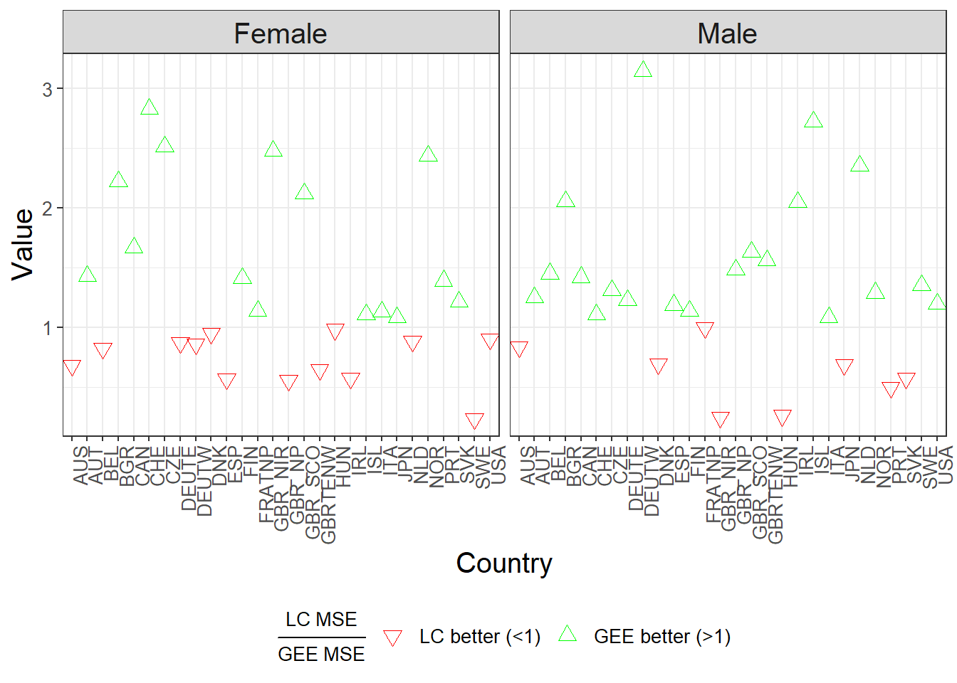
6. Conclusion

This analysis compares two approaches to forecasting mortality rates across 56 populations:

Lee–Carter Model (LC) – traditional demographic model.

Stochastic PCA–GEE Model – integrates dimension reduction and correlated error modeling.

The PCA–GEE model demonstrates improved forecasting accuracy for the majority of populations, particularly in capturing inter-age dependencies and stochastic dynamics.

7. Software and Packages

All analyses are conducted using the R statistical computing environment. Data manipulation and preprocessing are primarily performed with the data.table (Dowle et al. 2025) and dplyr (Wickham et al. 2023) packages, ensuring efficient handling of large mortality datasets. Data visualization and presentation of model results are carried out using ggplot2 (Wickham 2016).

Mortality data are obtained directly from the Human Mortality Database and imported into R via the HMDHFDplus package (Riffe 2015). The forecast package (R. Hyndman et al. 2024; R. J. Hyndman and Khandakar 2008) is employed to implement time series forecasting, specifically for estimating the stochastic evolution of mortality covariates.

For the Stochastic PCA–GEE model, the geepack package (Halekoh, Højsgaard, and Yan 2022; Yan and Højsgaard 2006) is used to fit Generalized Estimating Equations (GEEs) with an autoregressive correlation structure, capturing age-specific dependencies over time. Together, these tools provide a reproducible and extensible computational framework for analyzing and forecasting mortality dynamics.

References

Dowle, Matt, Arun Srinivasan, Jan Gorecki, Michael Chirico, Tom Short, Steve Lianoglou, Eduardo Almeida, Mark Yetman, Tyson Barrett, et al. 2025. Data.table: Extension of ‘Data.frame‘. https://CRAN.R-project.org/package=data.table.

Halekoh, Ulrich, Søren Højsgaard, and Jun Yan. 2022. Geepack: Generalized Estimating Equation Package. https://CRAN.R-project.org/package=geepack.

Hyndman, Rob J, and Yeasmin Khandakar. 2008. “Automatic Time Series Forecasting: The Forecast Package for r.” Journal of Statistical Software 27 (3): 1–22. https://doi.org/10.18637/jss.v027.i03.

Hyndman, Rob, George Athanasopoulos, Christoph Bergmeir, Gabriel Caceres, Leanne Chhay, Mitchell O’Hara-Wild, Fotios Petropoulos, Slava Razbash, Earo Wang, and Farah Yasmeen. 2024. Forecast: Forecasting Functions for Time Series and Linear Models. https://pkg.robjhyndman.com/forecast/.

Riffe, Tim. 2015. “Reading Human Fertility Database and Human Mortality Database Data into r.” TR-2015-004. Max Planck Institute for Demographic Research (MPIDR). https://doi.org/10.4054/MPIDR-TR-2015-004.

Wickham, Hadley. 2016. Ggplot2: Elegant Graphics for Data Analysis. Springer-Verlag New York. https://ggplot2.tidyverse.org.

Wickham, Hadley, Romain François, Lionel Henry, Kirill Müller, and Davis Vaughan. 2023. Dplyr: A Grammar of Data Manipulation. https://CRAN.R-project.org/package=dplyr.

Yan, Jun, and Søren Højsgaard. 2006. “The r Package Geepack for Generalized Estimating Equations.” Journal of Statistical Software 15 (2): 1–11. https://doi.org/10.18637/jss.v015.i02.